In previous posts, I have discussed methods for AB testing when we are interested only in the success rate of a design. It is often the case, however, that success rates don’t tell the whole story. In the case of banner adds, a successful conversion can lead to different amounts of reward. So while one design might give a high success rate but low reward per success, another design might have a low success rate but very high reward per success. We often care most about the expected reward of a design. If we just compare success rates and choose the design with the higher rate, we are not necessarily choosing the option with the higher expected reward. This post discusses how to do AB testing when the reward is limited to a set of fixed values. In particular, I demonstrate Bayesian computational techniques for determining:

1. the probability that one design gives a higher expected reward than another
2. confidence intervals for the percent difference in expected reward between two designs

A Motivating Example

To motivate the methods, let me give you a concrete use case. The Wikimedia Foundation (WMF) does extensive AB testing on their fundraising banners. Usually, the fundraising team only compares banners based on the fraction of users who made a donation (i.e. the success rate) because they are optimizing for a broad donor base.

As the foundation’s budget continues to grow, it has become more important increase the donation amount (i.e. the reward) per user as well. There are several factors that influence how much people give, including the ask string, the set of suggested donation amounts and the payment processor options. In order to increase the revenue per user in a principled way, it is necessary to AB test the expected donation amount per user for different designs.

Fundraising Banners offer a potential donor a small set suggested donation amounts. The image below shows a sample banner:

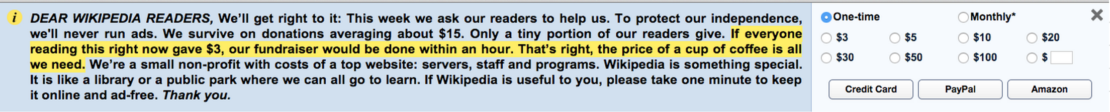
In this case, there are 7 discrete amount choices given. There is, of course, the implicit choice of $0, which a user exercises when they do not donate at all. In addition to the set of fixed choices, there is an option to enter a custom amount. In practice, only 2% of donors use the custom amount option. The image below gives an example of the empirical distribution over positive donation amounts from a recent test. Even visually, we get the impression that the fixed amounts dominate the character of the distribution.

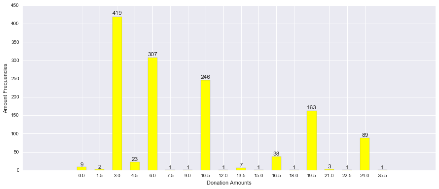
A clear choice for modeling the distribution over fixed donation amounts is the multinomial distribution. For modeling custom donations amounts, we could consider a continuous distribution over the set of positive numbers such as the log-normal distribution. Then we could model the distribution of over both fixed and custom amounts as a mixture between the two. For now, I will focus on just modeling the distribution over fixed amounts as they make up the vast majority of donations.

A primer on Bayesian Stats and Monte Carlo Methods

The key to doing Bayesian AB testing is to be able to sample from the joint posterior distribution \(\mathcal P \left({p_a, p_b | Data}\right)\) over the parameters \(p_a\), \(p_b\) governing the data generating distributions. Note that in the Bayesian setting, we consider the unknown parameters of our data generating distribution as random variables. In our case study, the parameters of interest are the vectors parameterizing the multinomial distributions over donation amounts for each banner.

You can get a numeric representation of the distribution over a function \(f\) of your parameters \(\mathcal P \left({ f(p_a, p_b) | Data}\right)\) by sampling from \(\mathcal P \left({p_a, p_b | Data}\right)\) and applying the function \(f\) to each sample \((p_a, p_b)\). With these numeric representations, it is possible to find confidence intervals over \(f(p_a, p_b|Data)\) and do numerical integration over regions of the parameter space that are of interest. In many cases, \(p_a\) is independent of \(p_b\). This is true in our fundraising example where users are split into non-overlapping treatment groups and the users in one treatment group do not affect users in the other. A common scenario where independence does not hold, even for separate treatment groups, is when the groups share a common pool of resources to choose from. To give a concrete example, say you are a hotel booking site. AB testing aspects of the booking process can be hard since booking outcomes between the two groups interact: if a user in one group books a vacancy, that booking is no longer available to any other user.

When the parameters of interest are independent, then the joint posterior distribution factors into the product of the individual posterior distributions:

\[ \mathcal P \left({ p_a, p_b | Data }\right) = \mathcal P \left({p_a | Data_a }\right) * \mathcal P \left({p_b | Data_b }\right) \]

This means we can we can generate a draw from the joint posterior distribution by drawing once from each individual posterior distribution.

Getting a Distribution Over the Expected Revenue per User

When running a banner we, observe data from a multinomial distribution parameterized by a vector \(p\) where \(p_i\) corresponds to the probability of getting a reward \(r_i\) from a user. We do not know the value of \(p\). Our goal is to estimate \(p\) based on the data we observe. The Bayesian way is not to find a point estimate of \(p\), but to define a distribution over \(p\) that captures our level uncertainty in the true value of \(p\) after taking into account the data that we observe.

The Dirichlet distribution can be interpreted as a distribution over multinomial distributions and is the way we characterize our uncertainty in \(p\). The Dirichlet distribution is also a conjugate prior of the multinomial distribution. This means that if our prior distribution over \(p\) is \(Dirichlet(\alpha)\), then after observing count \(c_i\) for each reward value, our posterior distribution over \(p\) is \(Dirichlet(\alpha + c)\).

The expected reward of a banner is given by \(R = p^T \cdot v\), the dot product between the vector of reward values and and the vector of probabilities over reward values. We can sample from the posterior distribution over the expected revenue per user by sampling from \(Dirichlet(\alpha + c)\) distribution and then taking a dot product between that sample and the vector of values \(v\).

From Theory to Code

To make the above theory more concrete, lets simulate running a single banner and use the ideas from above to model the expected return per user.

import numpy as np
from numpy.random import dirichlet
from numpy.random import multinomial
import matplotlib.pyplot as plt
import seaborn as sns


# Set of reward values for banner A 
values_a = np.array([0.0, 2.0, 3.0, 4.0])
# True probability of each reward for banner A 
p_a = np.array([0.4, 0.3, 0.2, 0.1])
# True expected return per user for banner A
return_a = p_a.dot(values_a.transpose())


def run_banner(p, n):
    """
    Simulate running a banner for n users
    with true probability vector over rewards p.
    Returns a vector of counts for how often each
    reward occurred.
    """
    return multinomial(n, p, size=1)[0]

    
def get_posterior_expected_reward_sample(alpha, counts, values, n=40000):
    """
    To sample from the posterior distribution over revenue per user,
    first draw a sample from the posterior distribution over the the
    vector of probabilities for each reward value. Second, take the dot product
    with the vector of reward values.
    """
    dirichlet_sample = dirichlet(counts + alpha, n)
    return dirichlet_sample.dot(values.transpose()) 

    
#lets assume we know nothing about our banners and take a uniform prior
alpha = np.ones(values_a.shape)
#simulate running the banner 1000 times
counts = run_banner(p_a, 1000)
# get a sample from the distribution over expected revenue per user
return_distribution = get_posterior_expected_reward_sample(alpha, counts, values_a)
# plot the posterior distribution agains the true value
fig, ax = plt.subplots()
ax.hist(return_distribution, bins = 40, alpha = 0.6, normed = True, label = 'n = 1000')
ax.axvline(x=return_a, color = 'b')
plt.xlabel('Expected Reward per User')

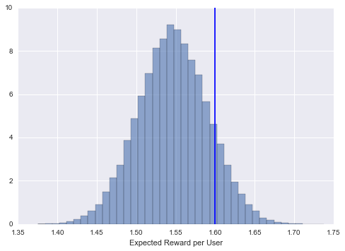
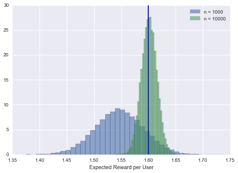
As we run the banner longer and more users enter the experiment, we should expect the distribution to concentrate around a tighter interval around the true return:

counts = run_banner(p_a, 10000)
return_distribution = get_posterior_expected_reward_sample(alpha, counts, values_a)
ax.hist(return_distribution, bins = 40, alpha = 0.6, normed = True, label = 'n = 10000')
ax.axvline(x=return_a, color = 'b')
ax.legend()
fig

Introducing Credible Intervals

One of the most useful things we can do with our posterior distribution over revenue per user is to build credible intervals. A 95% credible interval represents an interval that contains the true expected revenue per user with 95% certainty. The simplest way to generate credible intervals from a sample is to use quantiles. The quantile-based 95% probability interval is merely the 2.5% and 97.5% quantiles of the sample. We could get more sophisticated by trying to find the tightest interval that contains 95% of the samples. This may give quite different intervals than the quantile method when the distribution is asymmetric. For now we will stick with the quantile based method. As a sanity check, lets see if the method I describe will lead to 95% credible intervals that cover the true expected revenue per user 95% of the time. We will do this by repeatedly simulating user choices, building 95% credible intervals and recording if the interval covers the true expected revenue per user.

def get_credible_interval(dist, confidence):
    lower = np.percentile(dist, (100.0 - confidence) /2.0)
    upper = np.percentile(dist, 100.0 - (100.0 - confidence) /2.0)
    return lower, upper
       
def interval_covers(interval,true_value):
    """
    Check if the credible interval covers the true parameter
    """
    if interval[1] < true_value:
        return 0
    if interval[0] > true_value:
        return 0
    return 1

# Simulate multiple runs and count what fraction of the time the interval covers
confidence = 95
iters = 10000
cover_count = 0.0

for i in range(iters):
    #simulate running the banner
    counts = run_banner(p_a, 1000)
    # get the posterior distribution over rewards per user
    return_distribution = get_posterior_expected_reward_sample(alpha, counts, values_a)
    # form a credible interval over reward per user
    return_interval = get_credible_interval(return_distribution, confidence)
    # record if the interval covered the true reward per user
    cover_count+= interval_covers(return_interval, return_a)
    
print ("%d%% credible interval covers true return %.3f%% of the time" %(confidence, 100*(cover_count/iters)))

95% credible interval covers true return 95.000% of the time

Now you know how to generate the posterior distribution \(\mathcal P \left({R |Data}\right)\) over the expected revenue per user of a single banner and sample from it. This is the basic building block for the next section on comparing the performance of banners.

My Banner Is Better Than Yours

The simplest question one can ask in an AB test is: What is the probability that design A is better than design B? More specifically, what is the probability that \(R_a\), the expected reward of A, is greater than \(R_b\), the expected reward of B. Mathematically, this corresponds to integrating the joint posterior distribution over expected reward per user \(\mathcal P \left({R_a, R_b | Data}\right)\) over the region \(R_a > R_b\). Computationally, this corresponds to sampling from \(\mathcal P \left({R_a, R_b | Data}\right)\) and computing for what fraction of samples \((r_a, r_b)\) we find that \(r_a > r_b\). Since \(R_a\) and \(R_b\) are independent, we sample from \(\mathcal P \left({R_a, R_b | Data}\right)\) by sampling from \(\mathcal P \left({R_a | Data}\right)\) and \(\mathcal P \left({R_a | Data}\right)\) individually. In the code below, I introduce a banner B, simulate running both banners on 1000 users and then compute the probability of A being the winner.

# Set of returns for treatment B 
values_b = np.array([0.0, 2.5, 3.0, 5.0])
# True probability of each reward for treatment B
p_b = np.array([0.60, 0.10, 0.12, 0.18])
# True expected reward per user for banner B
return_b = p_b.dot(values_b)

# simulate running both banners
counts_a = run_banner(p_a, 1000)
return_distribution_a = get_posterior_expected_reward_sample(alpha, counts_a, values_a)
counts_b = run_banner(p_b, 1000)
return_distribution_b = get_posterior_expected_reward_sample(alpha, counts_b, values_b)

#plot the posterior distributions
plt.figure()
plt.hist(return_distribution_a, bins = 40, alpha = 0.4, normed = True, label = 'A')
plt.axvline(x=return_a, color = 'b')

plt.hist(return_distribution_b, bins = 40, alpha = 0.4, normed = True, label = 'B')
plt.axvline(x=return_b, color = 'g')
plt.xlabel('Expected Revenue per User')
plt.legend()

#compute the probability that banner A is better than banner B
prob_a_better = (return_distribution_a > return_distribution_b).mean()
print ("P(R_A > R_B) = %0.4f" % prob_a_better)

P(R_A > R_B) = 0.8514

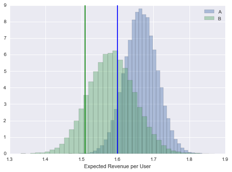
On this particular run, banner A and B did better than expected. Judging from the data we observe, we are 85% certain that banner A is better than banner B. Looking at one particular run, is not particularly instructive. For a given true difference \(R_a - R_b\) in expected rewards, the key factor that influences \(\mathcal P \left({R_a > R_b | Data}\right)\) is the sample size of the test. The following plot characterizes the the distribution over our estimates of \(\mathcal P \left({R_a > R_b | Data}\right)\) for different sample sizes.

results = []

for sample_size in range(500, 5000, 500):
    for i in range(1000):
        counts_a = run_banner(p_a, sample_size)
        return_distribution_a = get_posterior_expected_reward_sample(alpha, counts_a, values_a)
        counts_b = run_banner(p_b, sample_size)
        return_distribution_b = get_posterior_expected_reward_sample(alpha, counts_b, values_b)
        prob_a_better = (return_distribution_a > return_distribution_b).mean()
        results.append({'n':sample_size, 'p': prob_a_better})
        
sns.boxplot(x='n', y = 'p', data = pd.DataFrame(results))
plt.xlabel('sample size')
plt.ylabel('P(R_A > R_B)')

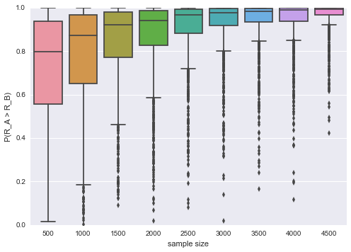
The plot illustrates an intuitive fact: the larger your sample, the more sure you will be about which banner is better. For the given ground truth distributions over rewards, we see that after 500 samples per treatment, the median certainty that banner A is better is 80%, with an interquartile range between 55% and 95% . After 4500 samples per treatment, the median certainty is 99.5 % and the interquartile range spans 96.8% and 99.93%. Being able to assign a level of certainty about whether one design is better than another is a great first step. The next question you will likely want to answer is how much better it is.

How much better?

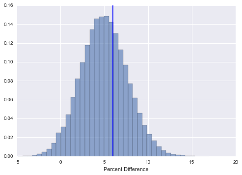
One approach, is to compare the absolute difference in expected rewards per user. If you need to communicate your results to other people, it is preferable to have a scale free measure of difference, such as the percent difference. In this section, I will describe how to build confidence intervals for the percent difference between designs. We can get a sample from the distribution over the percent difference \(\mathcal P \left({ 100 * \frac{R_a - R_b}{ R_b}| Data }\right)\), by taking a sample \((r_a, r_b)\) from \(\mathcal P \left({R_a, R_b| Data }\right)\) and applying the percent difference function to it. Once we have a distribution, we can from confidence intervals using quantiles as described above.

true_percent_difference = 100 * ((return_a - return_b) / return_b)

# simulate running both banners
counts_a = run_banner(p_a, 4000)
return_distribution_a = get_posterior_expected_reward_sample(alpha, counts_a, values_a)
counts_b = run_banner(p_b, 4000)
return_distribution_b = get_posterior_expected_reward_sample(alpha, counts_b, values_b)

#compute distribution over percent differences
percent_difference_distribution = 100* ((return_distribution_a - return_distribution_b) / return_distribution_b)


#plot the posterior distributions
plt.figure()
plt.hist(percent_difference_distribution, bins = 40, alpha = 0.6, normed = True)
plt.axvline(x=true_percent_difference, color = 'b')
plt.xlabel('Percent Difference')


#compute the probability that banner A is better than banner B
lower, upper = get_credible_interval(percent_difference_distribution, 95)
print ("The percent lift that A has over B lies in the interval (%0.3f, %0.3f) with 95%% certainty" % (lower, upper))

The percent lift that A has over B lies in the interval (-0.121, 10.285) with 95% certainty

To test the accuracy of the method, we can repeat the exercise from above of repeatedly generating confidence intervals and seeing if our x% confidence intervals cover the true percent difference x% of the time. You will see that they do:

# Simulate multiple runs and count what fraction of the time the interval covers
confidence = 95
iters = 10000
cover_count = 0.0

for i in range(iters):
    #simulate running the banner
    counts_a = run_banner(p_a, 4000)
    counts_b = run_banner(p_b, 4000)
    # get the posterior distribution over percent difference
    return_distribution_a = get_posterior_expected_reward_sample(alpha, counts_a, values_a)
    return_distribution_b = get_posterior_expected_reward_sample(alpha, counts_b, values_b)
    percent_difference_distribution = 100* ((return_distribution_a - return_distribution_b) / return_distribution_b)
    # get credible interval
    interval = get_credible_interval(percent_difference_distribution, confidence)
    # record if the interval covered the true reward per user
    cover_count+= interval_covers(interval, true_percent_difference)
    
print ("%d%% credible interval covers true percent difference %.3f%% of the time" %(confidence, 100*(cover_count/iters)))

95% credible interval covers true percent difference 94.940% of the time

That concludes my discussion of Bayesian techniques for AB testing designs where the reward per design is limited to a discrete set of values. I welcome feedback and questions in the comments section below.